Isotropy refers to the situation where the distance in Euclidean space in any direction is the same, leading to contour curves that are circular. While convenient, the hypothesis of isotropy is often untenable in geostatistic applications. To palliate to this, the easiest model adjustment one can consider is geometric anisotropy (see, e.g., Chilès and Delfiner (2012), section 2.5.2), whereby distance is elliptical. To achieve this, vectors of coordinate differences between locations \(i\) and \(j\), denoted \(\Delta_{ij}\boldsymbol{h} = (\Delta_{ij} \mathrm{lon}, \Delta_{ij} \mathrm{lat})^\top\), are multiplied by a matrix \(\mathbf{A}\) of the form \[\begin{align*}
\mathbf{A}(\boldsymbol{a}, \varphi) = \left(\begin{matrix} a_1 \cos \vartheta & a_1 \sin \vartheta \\ -a_2 \sin \vartheta & a_2 \cos \vartheta \end{matrix} \right).
\end{align*}\]
Code
#' Wrap angular component#'#' Due to identifiability issues in anisotropic models,#' we must restrict the angles to two quadrants.#' @param ang [double] angle in radians#' @param start [double] angle #' @return angles between \code{start} and \code{start} + \eqn{pi}#' @keywords internal#' @exportwrapAng <-function(ang, start =-pi/2) {stopifnot(length(start) ==1) (ang - start) %% pi + start}
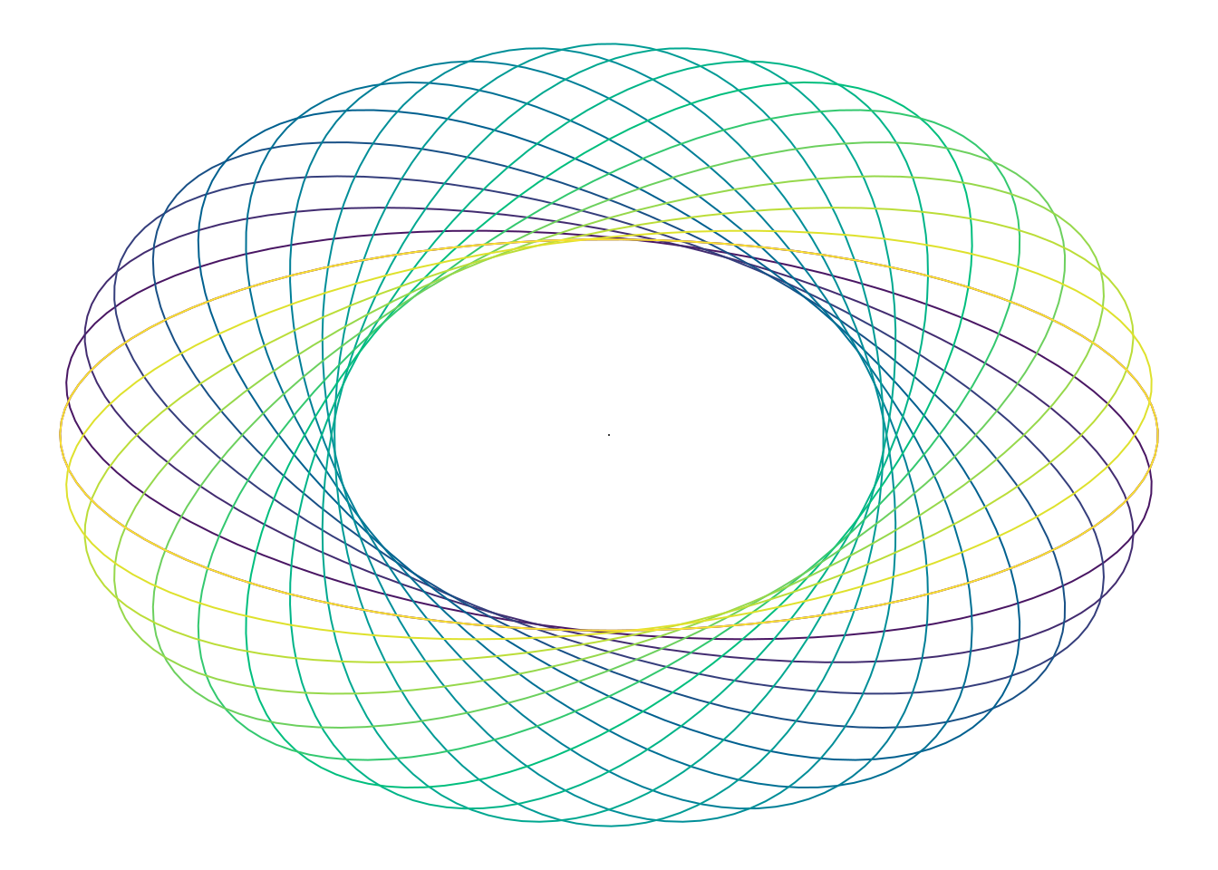
In a correlation model with a scale or range parameter, parameters \(a_1 \geq 1\) and \(a_2 \geq 1\) are not identifiable, so it is customary to fix one of them, e.g., \(a_1=1\). Such a parametrization leads to strong dependence between \(a_1\) and \(a_2\); also note that when \(a_1=a_2\), the model is isotropic and the angle \(\vartheta\) is not identifiable. We also restrict the angle \(\vartheta \in [0, \pi]\) or \(\vartheta \in [-\pi/2, \pi/2]\) since, as shown in Figure 1, it is sufficient to generate all elliptical patterns of interest.
Following Kazianka (2013), we use rather the parametrization \(r=a_2/a_1>0\) and set \(a_2=1\) to allow for an additional range parameter. This yields, for an exponential correlation, to a model of the form \(\exp\left\{-\phi\mathbf{h}^\top\mathbf{A}^\top\mathbf{A}\boldsymbol{h})^{1/2}\right\}\), where \[\begin{align*}
\mathbf{A} & = \begin{pmatrix}
1 & 0 \\
0 & r
\end{pmatrix}\begin{pmatrix}
\cos \vartheta & \sin \vartheta \\
- \sin \vartheta & \cos \vartheta
\end{pmatrix} \\
\mathbf{A}^\top\mathbf{A} &=
\begin{pmatrix}
\cos^2\vartheta + r^2 \sin^2 \vartheta & (1-r^2)\cos \vartheta \sin \vartheta \\
(1-r^2)\cos \vartheta \sin \vartheta & r^2 \cos^2 \vartheta + \sin^2 \vartheta\\
\end{pmatrix}, \qquad r \geq 1, \vartheta \in [0, \pi].
\end{align*}\] The identifiability constraints on the parameters are explained in Section 2.2 of Kazianka (2013): note for example that, since \(\cos^2(\vartheta) = \cos^2(\theta)\), \(\sin^2(\vartheta) = \sin^2(\theta)\) and \(\cos(\vartheta)\sin(\vartheta) = \cos(\theta)\sin(\theta)\) for \(\vartheta = \theta \pm \pi\), the angle needs to be restricted to the first and second, or the first and fourth quadrant. The decay parameter \(\phi\), also called reciprocal rate, controls the dependence decay in all directions.
Figure 1: Ellipses generated by different angles of anisotropy in the first and fourth quadrants, with fixed anisotropy ratio.
If the anisotropy ratio \(r \geq 1\) is very close to unity, the angle parameter \(\vartheta\) is unidentifiable. Since the likelihood is unaffected, acceptance will be determined solely by the prior and, since the latter is often uniform, angles can move around. If there is truly anisotropy, this in turn will lead to proposals for \(r\) to be rejected in subsequent sampling steps.
While it may be tempting to simulate the parameter value \(\vartheta \in [0, \pi)\) from a bounded distribution or map it to the real line, this is not sensible. Indeed, the two boundary values \(0\) and \(\pi\) give rise to the same ellipse as angles are equivalent as \(\vartheta - \vartheta_0 \mathrm{mod}(\pi) + \vartheta_0\), whereas for example a logit transformation would imply that the angles mapped to \(-\infty\) and \(\infty\) are very far. If we make proposals, the step size must also be adjusted since we could run in circle if the proposal variance is too large: we can restrict the latter to \(\pi/2\) and ideally would make the latter proportional to \(r\) for \(\vartheta\).
Anisotropic Gaussian processes and likelihood function
Consider an exponential covariance of the form \(\boldsymbol{Q}^{-1}=\tau\exp(-\phi\mathbf{D})\), with entries \(\mathrm{Cov}(Y_i, Y_j) = \tau\exp(-\phi d_{ij})\) for \(\mathbf{D}\) the \(n \times n\) distance matrix. The log likelihood for an \(n\) observation vector \(\boldsymbol{y}\) is \[\begin{align*}
\ell(\tau, \boldsymbol{\kappa}, r; y) \propto \frac{n}{2} \log(\tau) - \frac{1}{2}\log \left|\boldsymbol{Q}^{-1}\right| -\frac{\tau}{2} \boldsymbol{y}^\top \boldsymbol{Q}\boldsymbol{y}
\end{align*}\]
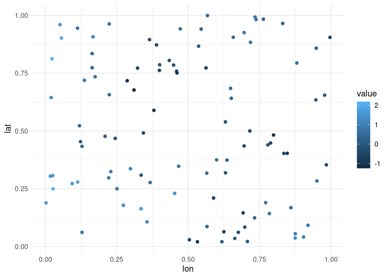
We first simulate some data from a mean-zero Gaussian process on the unit square with unit variance \(\tau=1\).
Figure 2: First realization of the Gaussian process with exponential correlation function on the unit square.
Next, we build a Gaussian log likelihood function incorporating with the geometric anisotropy and optimize the latter to see if we can retrieve the parameters.
Code
# Anisotropy matrix, using Kazianka (2013) parametrizationanisomat <-function(ang =0, r =1){ ang <- ang %% pistopifnot(r >=1) amat <-matrix(nrow =2, ncol =2) amat[1,1] <-cos(ang) amat[2,2] <- r*amat[1,1] amat[1,2] <-sin(ang) amat[2,1] <--r*amat[1,2]return(amat)}# Distance matrix geom_aniso <-function(coord, anisomat =diag(2)){stopifnot(is.matrix(coord), ncol(coord) ==2L) dmat <-matrix(0, nrow =nrow(coord),ncol =nrow(coord))stopifnot(is.matrix(anisomat), nrow(anisomat) ==2L,ncol(anisomat) ==2L)# Distance between longitude and latitude h <-apply(coord, 2, function(y){combn(y, 2, FUN =function(x){x[2]-x[1]})})dmat[lower.tri(dmat)] <-apply(h, 1, function(hv){sqrt(sum((anisomat %*% hv)^2))})dmat[upper.tri(dmat)] <-t(dmat)[upper.tri(dmat)]return(dmat)}# Check with Euclidean distancecoord_test <-matrix(runif(n =20L), ncol =2L)if(!isTRUE(all.equal(max(abs(as.matrix(dist(coord_test)) -geom_aniso(coord = coord_test))), 0,tol =1e-6))){print("Distance matrix is not correctly implemented.")}
# Gaussian log likelihood function loglik <-function( par, data, coord, index =NULL, otherpar){if(!is.null(index)){ tpar <-numeric(length =length(otherpar) +1L)stopifnot(is.integer(index),length(par) ==1L, index >=1L, index <=length(otherpar) +1L) tpar[-index] <- otherpar tpar[index] <- par } else{ tpar <- par }# reciprocal range phi <- tpar[1] r <- tpar[2] ang <- tpar[3] data <-as.matrix(data)# Exponential correlation matrix# Ecorr <- exp(-phi*geom_aniso(coord = coord, anisomat = anisomat(ang = ang, r = r))) Ecorr <-exp(-phi*mev::distg(loc = coord, rho = ang %% pi, scale = r))# Cholesky of precision matrix chol_Eprec <-backsolve(chol(Ecorr), diag(nrow(coord)))# Gaussian log likelihood loglik <-nrow(data)*sum(log(diag(chol_Eprec))) -0.5*sum(apply(data, 1, FUN =function(X){tcrossprod(X %*% chol_Eprec)}))return(loglik)}lb <-c(0, 1, 0)ub <-c(Inf, Inf, pi)start <-c(2, 1.5, pi/4)# loglik(par = start,# coord = coord,# dat = samp,# transform = FALSE)opt <- Rsolnp::solnp(pars = start,fun =function(par, ...){ -loglik(par, ...)},ineqfun =function(par, ...){par},ineqLB = lb,ineqUB = ub,data = samp,coord = coord,control =list(trace =0))if(opt$convergence ==0){cat("Parameter estimates at convergence\n")print(opt$pars)}
Parameter estimates at convergence
[1] 1.83 1.41 0.88
So far so good, nothing unexpected given the large sample size.
Prior specification
Kazianka (2013) proposes reference priors for all parameters, whereas Shen and Gelfand (2019) in their simulation study use independent priors with \(\vartheta \sim \mathsf{U}(0, \pi)\) for the angle, \(r \sim \mathsf{Ga}(1,1)\) and \(\phi \sim \mathsf{U}(6d_{\max}, 15d_{\max})\) for the decay parameter, where \(d_{\max}\) is the maximum Euclidean distance between sites.
For the decay parameter \(\phi\), the penalized complexity prior proposed by Fuglstad et al. (2019) in their Theorem 2.3 is, up to normalizing constant, Weibull with shape \(d/2\) and scale \(\lambda^{-d/2}\). Theorem 2.4 of Fuglstad et al. (2019) proposes to relate the hyperparameter \(\lambda\) to the tail probability for the range.
For \(r\), it may be useful to consider a prior that shrinks toward 1, which corresponds to the isotropic case. If we wanted to allow for a point mass at unity, we could use a spike-and-slab prior (Madigan and Raftery 1994)\(r-1 \sim p_0\mathsf{I}(r=0) + (1-p_0)\mathsf{St}_{+}(1)\) and implement a reversible jump algorithm (Green 1995). Any distribution that is unbounded at the origin, for example a Gamma with shape less than one, would also work as prior for the continuous part if we shift it by one.
logpriors <-function( par,index =NULL, otherpar, ...){if(!is.null(index)){ tpar <-numeric(length(otherpar) +1L)stopifnot(is.integer(index),length(par) ==1L, index >=1L, index <=length(otherpar) +1L) tpar[-index] <- otherpar tpar[index] <- par } else{ tpar <- par }# reciprocal range phi <- tpar[1] r <- tpar[2] ang <- tpar[3] %% pi lambda <-3dunif(ang, min =0, max = pi, log =TRUE) +# prior for angle#dgamma(x = phi, shape = 1, scale = 1, log = TRUE) + dweibull(x = phi, shape =1, scale = lambda, log =TRUE) +# PC prior for exponential range, need to fix 'lambda'# I(r==1)*(log(2) + dt(x = r-1, df = 2, log = TRUE)) + # slab prior# dbinom(x = r == 1, size = 1, prob = 0.2, log = TRUE) # prior for augmentation Z dgamma(x = r-1, scale =1, shape =1, log =TRUE)}
The log penalized complexity prior with \(\lambda = 3\) is -1.77 (-2.77) at distance 2 (respectively 5).
Posterior sampling via Markov chain Monte Carlo methods
We begin with a simple Markov chain Monte Carlo sample updating each parameter in turn using random walk Metropolis–Hastings, with a circular proposal for the angle modulo pi.
# MCMC samplersource("mcmc_helpers.R")source("truncated_normal.R")B <-1e4Lburnin <-1e3Lnpar <-3Llbound <-c(0, 1, -Inf)posterior <-matrix(nrow = B, ncol = npar)acceptance <-rep(0L, npar) # number of moves acceptedattempts <-rep(0L, npar) # number of proposalspar_cur <- start # initial value for the parametercolnames(posterior) <- names <-c("phi", "r", "ang")sd_prop <-rep(0.3, npar) # std. dev of proposalsfor(i inseq_len(B + burnin)){ ind <-pmax(1, i - burnin) # store values, then restart the counter# Run random walkfor(j inseq_along(par_cur)){ posterior[ind, j] <-univariate_rw_update(par_curr = par_cur[j], # current value of the parameterpar_name ="par", # name of the variable loglik = loglik, # log-likelihood functionlogprior = logpriors, # log prior functionsd_prop = sd_prop[j], lb = lbound[j],data = samp, # additional arguments passed to the functioncoord = coord,otherpar = par_cur[-j],index = j) if(posterior[ind, j] != par_cur[j]){ acceptance[j]<- acceptance[j] +1L #increment counter if move is accepted } attempts[j] <- attempts[j] +1L# Save current value posterior[ind, j] -> par_cur[j] }if(i %%100& i < burnin){# Adapt proposal every 100 iterationsfor(j inseq_along(par_cur)){ out <-adaptive(attempts = attempts[j], acceptance = acceptance[j], sd.p = sd_prop[j])# The function may return the values, or else change counters# We copy these sd_prop[j] <- out$sd acceptance[j] <- out$acc attempts[j] <- out$att } }}posterior[,3] <- posterior[,3] %% pi
With a large anisotropy ratio, we see that \((r, \phi)\) are strongly correlated. Shen and Gelfand (2019), who used Metropolis–Hastings steps to draw parameters one at the time, using truncated Gaussian proposals on \(\mathbb{R}_{+}\) for \(r\) (even if the latter is constrained), log-Gaussian proposal for \(\phi\) and Gaussian (mod \(\pi\)) for the angle \(\vartheta\), noted that the pair \((\vartheta, r)\) was strongly correlated a posteriori and should be updated jointly.
# Acceptance ratioprint(acceptance/attempts)
[1] 0.22 0.23 0.21
# Correlation between posterior drawscor(posterior)
       phi      r    ang
phi  1.000 -0.662  0.083
r   -0.662  1.000 -0.061
ang  0.083 -0.061  1.000
# Percentage of effective sample relative to number of simulationscoda::effectiveSize(posterior)/B
  phi     r   ang
0.060 0.063 0.207
Reparametrization and joint updates
We consider in the sequel the case where \(r > 1\) (i.e., no point mass). To alleviate problems with correlation, we consider joint updates to all parameters, but doing sequential updates after a change of variable.
The change of variable with \(\kappa_1 = \phi \cos \vartheta\), \(\kappa_2 = \phi\sin \vartheta\) with support \(\mathbb{R}_{+} \times [0, \pi] \mapsto \mathbb{R} \times \mathbb{R}_{+}\) is bijective with Jacobi matrix
and Jacobian \(|\mathrm{J}|=\phi\). The inverse transformation \(\phi = (\kappa_1^2 + \kappa_2^2)^{1/2}\) and \(\vartheta = \mathrm{arccot}(\kappa_1/\kappa_2)\) with Jacobi matrix \[\begin{align*}
\mathrm{J}=
\begin{pmatrix}
\kappa_1(\kappa_1^2 + \kappa_2^2)^{-1/2} & \kappa_2(\kappa_1^2+\kappa_2^2)^{-1}\\
\kappa_2(\kappa_1^2 + \kappa_2^2)^{-1/2} & -\kappa_1(\kappa_1^2+\kappa_2^2)^{-1} \end{pmatrix}
\end{align*}\] and Jacobian \((\kappa_1^2 + \kappa_2^2)^{-1/2}\). The uniform-penalized complexity priors for \((\phi, \vartheta)\), with the Jacobian, becomes in the transformed scale, \[\begin{align*}
p(\kappa_1, \kappa_2; \lambda) \propto \lambda (\kappa_1^2 + \kappa_2^2)^{-1/2}\exp\left\{-\lambda(\kappa_1^2 + \kappa_2^2)^{1/2}\right\}
\end{align*}\] and the log-prior derivative with respect to \(\kappa_j (j=1, 2)\) are \[\begin{align*}
\frac{\partial \log p(\kappa_1, \kappa_2; \lambda)}{\partial \kappa_j} = -\frac{\kappa_j}{\kappa_1^2 + \kappa_2^2} \left\{1+ \lambda (\kappa_1^2 + \kappa_2^2)^{1/2}\right\}
\end{align*}\] With the reparametrization, the squared Euclidean distance becomes \[\begin{align*}
d_{ij}^2 &=
\Delta_{ij}\boldsymbol{h}^\top \mathbf{A}^\top\mathbf{A}\Delta_{ij}\boldsymbol{h}\\
&= (\kappa_1^2+r^2\kappa_2^2) \Delta_{ij}^2 \mathrm{lon} + (r^2\kappa_1^2+\kappa_2^2) \Delta_{ij}^2 \mathrm{lat} +2 \kappa_1\kappa_2(1-r^2) \Delta_{ij} \mathrm{lon} \Delta_{ij} \mathrm{lat}
\end{align*}\]
Let \(\boldsymbol{\theta}_{\text{curr}} = (\boldsymbol{\kappa}_{\text{curr}}^\top, r_{\text{curr}})^\top\) denote the current parameter value. We calculate the gradient with respect to all three parameters to obtain proposal location parameter \(\boldsymbol{\mu}_{\text{prop}} = \boldsymbol{\theta}_{\text{curr}} + \delta\mathbf{M}\nabla \left.\ell(\boldsymbol{\theta})\right|_{\boldsymbol{\theta} = \boldsymbol{\theta}_{\text{curr}}}\), where \(\delta>0\) a damping parameter and \(\mathbf{M}\) a mass matrix. The latter here is taken to be proportional to the initial Markov chain run covariance matrix; good alternatives for \(\mathbf{M}\) would include the inverse of the negative log hessian at the maximum a posterior. We simulate a multivariate truncated Gaussian proposal for \(\boldsymbol{\theta}\) on \(\mathbb{R} \times \mathbb{R}_{+} \times [1, \infty)\) with location \(\boldsymbol{\mu}_{\text{prop}}\) and covariance matrix \(\mathbf{M}\). For the MALA, we additionally need to compute the reverse move formed by taking a step from a multivariate truncated Gaussian with location parameter \(\boldsymbol{\mu}_{\text{curr}} = \boldsymbol{\theta}_{\text{prop}}+ \delta\mathbf{M}\nabla \left.\ell(\boldsymbol{\theta})\right|_{\boldsymbol{\theta} = \boldsymbol{\theta}_{\text{prop}}}\).
To calculate the gradient for a MALA update or quadratic approximation, we follow the derivations in Appendix A.2 from Dyrrdal et al. (2014). The gradient with respect to parameters \(\tau, \kappa_1, \kappa_2, r\) involves matrix derivatives: using formulas 43 and 59 of the Petersen and Pedersen (2012) Matrix Cookbook, we have \(\partial \log |\mathbf{X}| / \partial \theta = \mathrm{tr}(\mathbf{X}^{-1} \partial \mathbf{X}/\partial \theta)\) whereas \(\partial \mathbf{X}^{-1}/\partial \theta = - \mathbf{X}^{-1} \partial \mathbf{X}/ \partial \theta \mathbf{X}^{-1}\).
The derivative of the exponential correlation matrix with respect to a generic parameter \(\theta\) is simply \(\partial \exp(-\mathbf{D})/\partial \theta = -\mathbf{D}_\theta\odot\exp(-\mathbf{D})\), where \(\odot\) denotes the Hadamard (i.e., element-wise) product. The mixed second derivative with respect to \(\theta_k\theta_l\) of the correlation function is \(\big( \mathbf{D}_{\theta_k}\odot \mathbf{D}_{\theta_l} -\mathbf{D}_{\theta_k \theta_l}) \odot \exp(-\mathbf{D})\). Additional terms can be found using the product rule and interchanging the trace and derivative since both are linear operators.
Simple derivations give \[\begin{align*}
\frac{\partial d_{ij}}{\partial \kappa_1} = \frac{1}{2d_{ij}}\left\{2\kappa_1 \Delta_{ij}^2 \mathrm{lon} + 2r^2\kappa_1\Delta_{ij}^2 \mathrm{lat} +2 \kappa_2(1-r^2) \Delta_{ij} \mathrm{lon} \Delta_{ij} \mathrm{lat}\right\}
\end{align*}\] and similarly for \(\partial d_{ij}/\partial \kappa_2\). Writing \(\boldsymbol{\Sigma}\) for the exponential covariance and \(\boldsymbol{\Sigma}_{\kappa}\) for the gradient with respect to \(\kappa\), we get the log-likelihood gradient (Dyrrdal et al. 2014)\[\begin{align*}
\frac{\partial \ell}{\partial \kappa} = -\frac{n}{2} \mathrm{tr}\left(\boldsymbol{\Sigma}^{-1}\boldsymbol{\Sigma}_{\kappa} \right)-\frac{1}{2} \sum_{i=1}^n \boldsymbol{y}_i^\top \boldsymbol{\Sigma}^{-1} \left[-\boldsymbol{\Sigma}_{\kappa}\right] \boldsymbol{\Sigma}^{-1}\boldsymbol{y}_i.
\end{align*}\]
anisomat2 <-function(kappa, r =1){stopifnot(r >=1) amat <-matrix(nrow =2, ncol =2) amat[1,1] <- kappa[1] amat[2,2] <- r*kappa[1] amat[1,2] <- kappa[2] amat[2,1] <--r*kappa[2]return(amat)}# Distance matrix Dmat <-function(kappa, r, coord){geom_aniso(coord = coord,anisomat =anisomat2(kappa = kappa, r = r))}Dmat_deriv <-function(kappa, r, coord, index =1L){stopifnot(is.matrix(coord), ncol(coord) ==2L, index %in%1:3) dmat <-matrix(0, nrow =nrow(coord),ncol =nrow(coord)) h <-apply(coord, 2, function(y){combn(y, 2, FUN =function(x){x[2]-x[1]})}) aniso <-anisomat2(kappa = kappa, r = r)if(index ==1L){ #kappa1dmat[lower.tri(dmat)] <-apply(h, 1, function(hv){0.5/sqrt(sum((aniso %*% hv)^2))*#1/d (2*kappa[1]*hv[1]^2+2*r^2*kappa[1]*hv[2]^2+2*kappa[2]*(1-r^2)*hv[1]*hv[2])}) } elseif(index ==2L){ #kappa2 dmat[lower.tri(dmat)] <-apply(h, 1, function(hv){0.5/sqrt(sum((aniso %*% hv)^2))*#1/d (2*r^2*kappa[2]*hv[1]^2+2*kappa[2]*hv[2]^2+2*kappa[1]*(1-r^2)*hv[1]*hv[2])}) } elseif(index ==3L){ #r dmat[lower.tri(dmat)] <-apply(h, 1, function(hv){ r/sqrt(sum((aniso %*% hv)^2))*#1/d (kappa[2]^2*hv[1]^2+ kappa[1]^2*hv[2]^2-2*kappa[1]*kappa[2]*hv[1]*hv[2])}) }dmat[upper.tri(dmat)] <-t(dmat)[upper.tri(dmat)]return(dmat)}logprior <-function(pars, lambda =3){ kappa <- pars[1:2] r <- pars[3]dgamma(x = r-1, scale =1, shape =1, log =TRUE) +log(lambda) -0.5*log(sum(kappa^2)) - lambda*sqrt(sum(kappa^2))}grad_logprior <-function(pars, lambda =3){ kappa <- pars[1:2] r <- pars[3]c(- kappa/(sum(kappa^2))*(1+lambda*sqrt(sum(kappa^2))),-1) # derivative of exponential prior for r}loglik <-function(pars, data, coord){ kappa <- pars[1:2] r <- pars[3] Ecorr <-exp(-Dmat(coord = coord, kappa = kappa, r = r))# Cholesky of precision matrix chol_Eprec <-backsolve(chol(Ecorr), diag(nrow(coord)))# Gaussian log likelihood loglik <-nrow(data)*sum(log(diag(chol_Eprec))) -0.5*sum(apply(data, 1, FUN =function(X){tcrossprod(X %*% chol_Eprec)}))return(loglik)}# Gradient with respect to kappagrad_loglik <-function(pars, data, coord){ kappa <- pars[1:2] r <- pars[3] E <-exp(-Dmat(coord = coord, kappa = kappa, r = r)) Q <-solve(E) Eprime1 <--Dmat_deriv(kappa = kappa, r = r, coord = coord, index =1) * E Eprime2 <--Dmat_deriv(kappa = kappa, r = r, coord = coord, index =2) * E Eprime3 <--Dmat_deriv(kappa = kappa, r = r, coord = coord, index =3) * Ec(-0.5*sum(apply(data, 1, function(X){ -t(X) %*% Q %*% Eprime1 %*% Q %*% X})) -nrow(data)/2*sum(diag(Q %*% Eprime1)),-0.5*sum(apply(data, 1, function(X){ -t(X) %*% Q %*% Eprime2 %*% Q %*% X})) -nrow(data)/2*sum(diag(Q %*% Eprime2)),-0.5*sum(apply(data, 1, function(X){ -t(X) %*% Q %*% Eprime3 %*% Q %*% X})) -nrow(data)/2*sum(diag(Q %*% Eprime3)))}# Check analytical gradient with numerical differentiationmle <-with(opt, c(pars[1]*cos(pars[3]), pars[1]*sin(pars[3]), pars[2]))all.equal(numDeriv::grad(loglik, x =c(1, 2, 1.5),data = samp,coord = coord),grad_loglik(pars =c(1, 2, 1.5), data = samp, coord = coord))
[1] TRUE
# Use the previous run to get a weighting matrix for proposaltpars_mcmc <-cbind( posterior[,1]*cos(posterior[,3]), posterior[,1]*sin(posterior[,3]), posterior[,2])pars_cov <-cov(tpars_mcmc)# Proposal for the joint vector (kappa, r)rprop <-function(pars, pars_cov, damp =1, data, coord){# hessian_prop <- numDeriv::jacobian(# func = function(pars, data, coord){# grad_loglik(pars = pars, coord = coord, data = data) + # grad_logprior(pars = pars)},# x = par, # data = data, # coord = coord,# method = "complex") pars_curr <- pars mu_prop <- pars_curr + damp * pars_cov %*% (grad_loglik(pars = pars_curr, data = data, coord = coord) +grad_logprior(pars = pars_curr) ) pars_prop <- TruncatedNormal::rtmvnorm(n =1,mu = mu_prop,sigma = pars_cov,lb =c(-Inf, 0, 1)) mu_curr <- pars_prop + damp * pars_cov %*% (grad_loglik(pars = pars_prop, data = data, coord = coord) +grad_logprior(pars = pars_prop))return(list(pars_prop = pars_prop,pars_curr = pars_curr,mean_prop = mu_prop,mean_curr = mu_curr,pars_cov = pars_cov))}# Calculate the Metropolis-Hastings ratio for MALAmhkernelratio <-function(list_mala,log =TRUE){with(list_mala, TruncatedNormal::dtmvnorm(x = pars_curr, mu = mean_curr, sigma = pars_cov,lb =c(-Inf, 0, 1),log =TRUE) - TruncatedNormal::dtmvnorm(x = pars_prop, mu = mean_prop, sigma = pars_cov,lb =c(-Inf, 0, 1),log =TRUE) )}
We can now build a sampler incorporating all of the ingredients discussed above.
Unsurprisingly, the sampler is much slower than before as we now need to evaluate gradients (for both the proposal and reverse move), as well as several matrix inverses.
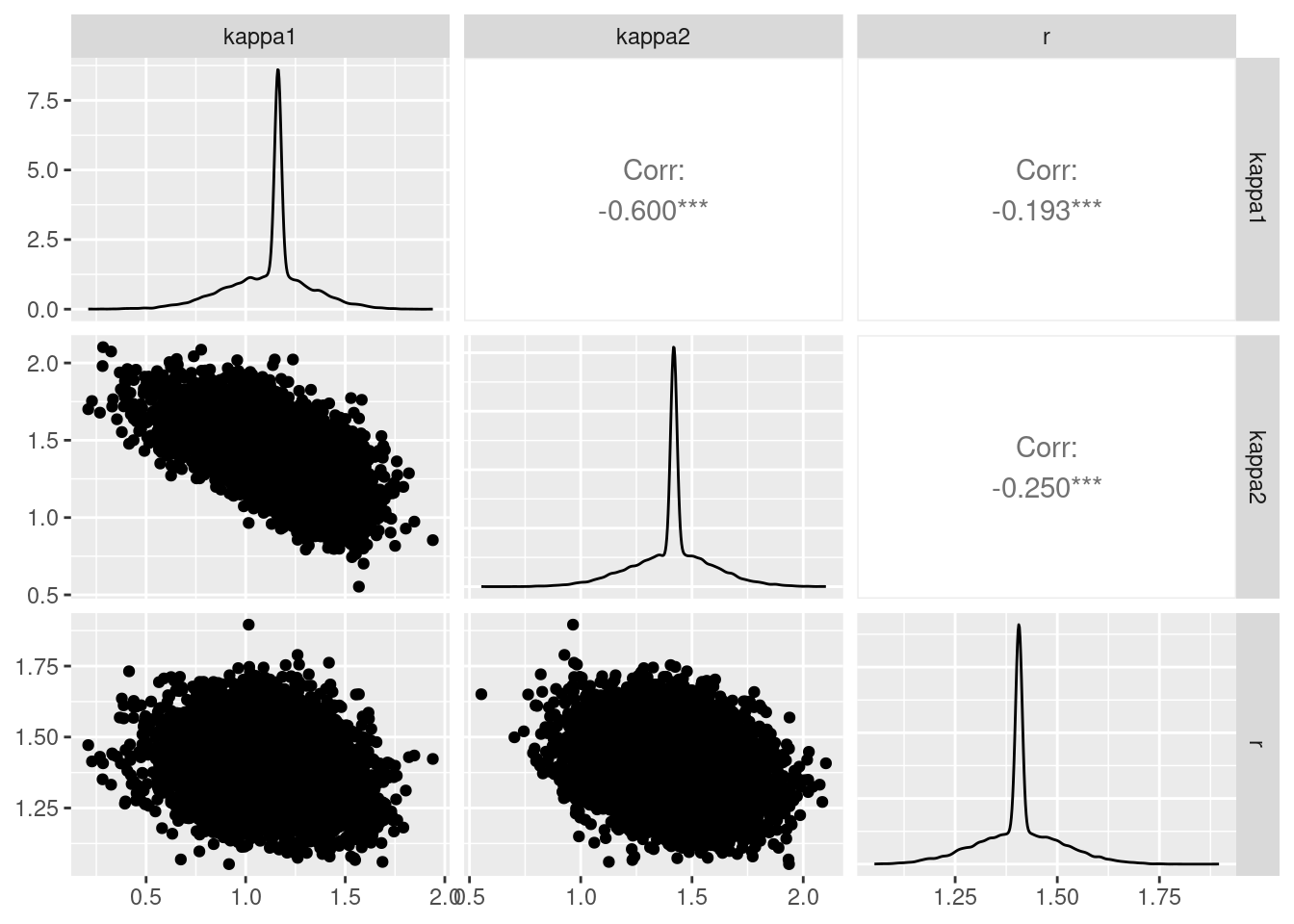
With the MALA sample, 68% of the joint proposals are accepted with near zero autocorrelation: the effective sample size relative to the total number of simulated values for \(\kappa_1\) is, e.g., 104%. However, the marginal posterior density suggests that the sampler gets stuck and returns to the mode.
Figure 4: Traceplots of Markov chains for reparametrized model.
Assessing directions for circular data
Summary statistics for circular processes of interest include the mean angle and variance length, defined in terms of sin and cosine of the angles, as follows \[\begin{align*}
\overline{\sin} &= n^{-1}\sum_{i=1}^n \sin(\vartheta_i),\\
\overline{\vphantom{i}\cos} &= n^{-1}\sum_{i=1}^n \cos(\vartheta_i),\\
\overline{\vartheta} &= \arctan \left(\overline{\sin}/\overline{\vphantom{i}\cos}\right), \\
\mathsf{var}(\vartheta) & = 1 - \sqrt{\overline{\sin}^2 + \overline{\vphantom{i}\cos}^2}
\end{align*}\] For summary statistics, we would need ignore all angles generated when \(r=1\), should there be a point mass for the isotropic case.
Code
#' Angular mean and variance length for processes mod pi#' #' Since the process is defined mod pi, we shift angles by start#' and multiply them by 2 before calculating the angular mean and variance.#' Due to the back-transformation, the maximum variance length that can be achieved#' is 1/2.#' @inheritParams wrapAng#' @param weights [double] vector of weights#' @return a list with components#' \describe{#' \item{\code{mean}}{mean angle, between \code{start} and \code{start} + \eqn{pi}}#' \item{\code{varl}}{variance length}#' }#' @keywords internal#' @exporsummaryAng <-function(ang, start, weights =rep(1, length(ang))) {# Put angles back on [0, 2pi]stopifnot(length(weights) ==length(ang),length(start) ==1L) ang <-2*(wrapAng(ang, start = start) - start) msin <-sum(weights*sin(ang))/sum(weights) mcos <-sum(weights*cos(ang))/sum(weights)list(mean =wrapAng(atan(msin/mcos)/2+ start, start = start),varl =1-sqrt(msin^2+ mcos^2) )}
For example, we can convert the posterior samples back into angle and compute the mean direction.
theta_post <-atan2(y = posterior2[,2], x = posterior2[,1])mean(theta_post)
Dyrrdal, Anita V., Alex Lenkoski, Thordis L. Thorarinsdottir, and Frode Stordal. 2014. “Bayesian Hierarchical Modeling of Extreme Hourly Precipitation in Norway.”Environmetrics 26 (2): 89–106. https://doi.org/10.1002/env.2301.
Fuglstad, Geir-Arne, Daniel Simpson, Finn Lindgren, and Håvard Rue. 2019. “Constructing Priors That Penalize the Complexity of Gaussian Random Fields.”Journal of the American Statistical Association 114 (525): 445–52. https://doi.org/10.1080/01621459.2017.1415907.
Green, Peter J. 1995. “Reversible Jump Markov Chain Monte Carlo Computation and Bayesian Model Determination.”Biometrika 82 (4): 711–32. https://doi.org/10.1093/biomet/82.4.711.
Kazianka, Hannes. 2013. “Objective Bayesian Analysis of Geometrically Anisotropic Spatial Data.”Journal of Agricultural, Biological, and Environmental Statistics 18 (4): 514–37. https://doi.org/10.1007/s13253-013-0137-y.
Madigan, David, and Adrian E. Raftery. 1994. “Model Selection and Accounting for Model Uncertainty in Graphical Models Using Occam’s Window.”Journal of the American Statistical Association 89 (428): 1535–46. https://doi.org/10.1080/01621459.1994.10476894.
Shen, Y., and A. E. Gelfand. 2019. “Exploring Geometric Anisotropy for Point-Referenced Spatial Data.”Spatial Statistics 32: 100370. https://doi.org/10.1016/j.spasta.2019.100370.
Citation
BibTeX citation:
@online{belzile2023,
  author = {Belzile, Léo},
  title = {Bayesian Modelling of Geometric Anisotropy},
  date = {2023-08-02},
  url = {https://lbelzile.bitbucket.io/posts/geometric-aniso/},
  langid = {en}
}