Strategies for Markov chain Monte Carlo algorithms
Different strategies for the design of Markov chain Monte Carlo using random walk Metropolis proposals, Metropolis-adjusted Langevin algorithm. We consider a simple beta-binomial scenario with parameter transformations.
In Bayesian modelling, posterior samples are often sampled using Markov chain Monte Carlo methods, notably via Metropolis–Hastings steps. The purpose of this vignette is to showcase generic functions to sampling updates, in addition to step performing Metropolis–adjusted Langevin algorithm (MALA) and quadratic approximations that utilize both the gradient and Hessian matrix and thus do not require tuning of the variance of the proposal.
Metropolis–Hastings algorithm
Let \(\ell(\theta)\) and \(\pi(\theta)\) denote the likelihood and prior density, respectively. Random walk Metropolis–Hastings algorithm is one of the most popular and generic Markov chain Monte Carlo sampler (Robert and Casella 2004). The underlying idea is simple: given a current value for the parameter of interest \(\theta^{\text{curr}}\), we draw a proposal from a kernel \(q\), say \(\theta^{\text{prop}}\) and calculate the acceptance ratio \[
\alpha = \frac{\exp\{\ell(\theta^{\text{prop}})\} \pi(\theta^{\text{prop}})}{\exp\{\ell(\theta^{\text{curr}})\}\pi(\theta^{\text{curr}})} \frac{q(\theta^{\text{curr}}; \theta^{\text{prop}})}{q(\theta^{\text{prop}}; \theta^{\text{curr}})};
\tag{1}\] the probability of accepting the move is \(\max\{1, \alpha\}\). In practice, we compute every term on the log scale to avoid numerical overflow.
For the purpose of illustration, we generate fake data from a Bernoulli distribution with probability of success \(p=0.2\) and use a conjugate Beta prior: in this case, the posterior distribution will be known exactly.
One of the most popular proposal for Metropolis–Hastings is a Gaussian random walk: the proposal is a normal kernel centered at the current value \(\theta^{\text{prop}} = \theta^{\text{curr}}+\tau Z\) where \(Z \sim \mathsf{No}(0, 1)\). Since the normal density is symmetric, the ratio in the second fraction of Equation 1 is 1. The percentage of moves that get accepted depends on the variance of the proposal, \(\tau^2\): if the latter is too small, the acceptance rate will be high but exploration will be slow, whereas if it is too large, most moves will be rejected. We can tune the variance term \(\tau^2\) to target an acceptance rate of about 0.48 in the univariate case and 0.234 for multivariate proposals Sherlock (2013). We can use the history of the Markov chain to tune this parameter by multiplying \(\tau\) by a positive constant larger (respectively smaller) if the acceptance rate is too high (too low). To satisfy diminishing adaptation, we only adapt during the burn-in period, which consists of the initial steps of the MCMC for which the history of the chain isn’t saved. This period is meant to ensure convergence to the stationary distribution.
To check that the algorithm is well-defined, we can remove the log likelihood component and run the algorithm: if it is well implemented, the resulting draws should be drawn from the prior (Green 1995).
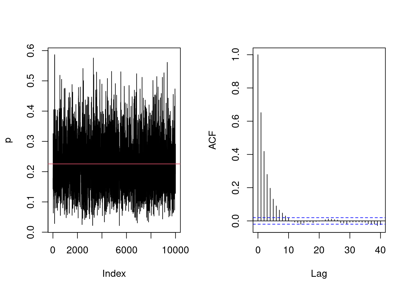
par_cont <-numeric(B)acceptance <-0# number of moves acceptedattempts <-0# number of proposalspar_cur <-runif(1) # initial value for the parametersd_prop <-0.45# std. dev of proposalfor(i inseq_len(B + burnin)){ ind <-pmax(1, i - burnin) # store values, then restart the counter# Run random walk par_cont[ind] <-univariate_rw_update(par_curr = par_cur, # current value of the parameterpar_name ="p", # name of the variable loglik = loglik, # log-likelihood functionlogprior = logprior, # log prior functionsd_prop = sd_prop, data = data) # additional arguments passed to the functionif(par_cont[ind] != par_cur){ acceptance <- acceptance +1L #increment counter if move is accepted } attempts <- attempts +1L# Save current value par_cont[ind] -> par_curif(i %%100& i < burnin){# Adapt proposal every 100 iterations out <-adaptive(attempts = attempts, acceptance = acceptance, sd.p = sd_prop,target =0.44)# The function may return the values, or else change counters# We copy these sd_prop <- out$sd acceptance <- out$acc attempts <- out$att }}# Plot the Markov chain and the correlogrampar(mfrow =c(1,2))plot(par_cont, type ="l", ylab ="p")abline(h =mean(par_cont), col =2)acf(par_cont, main ="")coda::effectiveSize(par_cont)/B
 var1
0.201
While the acceptance rate is seemingly in line with our expectations, the fact that the probability of success \(p\) lies in the unit interval may lead to many proposals being discarded if we are very close to the origin, as any negative value of \(p\) leads to zero likelihood. The effective sample size is 15% of \(B\) replications.
Bounded parameters
Parameter transformation: If the parameter is bounded in the interval \((a,b)\), where \(-\infty \leq a < b \leq \infty\), we can consider a bijective transformation \(\vartheta \equiv t(\theta): (a,b) \to \mathbb{R}\) with differentiable inverse. The log density of the transformed variable, assuming it exists, is \[\begin{align*}
f_\vartheta(\vartheta) = f_{\theta}\{t^{-1}(\vartheta)\} \left| \frac{\mathrm{d}}{\mathrm{d} \vartheta} t^{-1}(\vartheta)\right|
\end{align*}\] Section 52 of the STAN reference manual (Stan Development Team 2018) details the use of the following transformations for finite \(a, b\) in the software:
if \(\theta \in (a, \infty)\) (lower bound only), then \(\vartheta = \log(\theta-a)\) and \(f_{\vartheta}(\vartheta)=f_{\theta}\{\exp(\vartheta) + a\}\cdot \exp(\vartheta)\)
if \(\theta \in (-\infty, b)\) (upper bound only), then \(\vartheta = \log(b-\theta)\) and \(f_{\vartheta}(\vartheta)=f_{\theta}\{b-\exp(\vartheta)\}\cdot \exp(\vartheta)\)
if \(\theta \in (a, b)\) (both lower and upper bound), then \(\vartheta = \mathrm{logit}\{(\theta-a)/(b-a)\}\) and \(f_{\vartheta}(\vartheta)=f_{\theta}\{a+(b-a) \mathrm{expit}(\vartheta)\}\cdot (b-a)\cdot \mathrm{expit}(\vartheta)\cdot\{1-\mathrm{expit}(\vartheta)\}\)
To guarantee that our proposals fall in the support of \(\theta\), we can thus run a symmetric random walk proposal on the transformed scale by drawing \(\vartheta^{\text{prop}} \sim \vartheta^{\text{curr}}+\tau Z\) where \(Z\sim\mathsf{No}(0, 1)\). Due to the transformation, the kernel ratio now contains the Jacobian.
Truncated proposals: as an alternative, we can simulate \(\theta^{\text{prop}} \sim \mathsf{TNo}(\vartheta^{\text{curr}}, \tau^2, a, b)\). The density of the truncated normal distribution is \[\begin{align*}
f(x; \mu, \tau, a, b) = \tau^{-1}\frac{\phi\left(\frac{x-\mu}{\tau}\right)}{\Phi\{(b-\mu)/\tau\}-\Phi\{(a-\mu)/\tau\}}.
\end{align*}\] where \(\phi(\cdot), \Phi(\cdot)\) are respectively the density and distribution function of the standard normal distribution. While the benefit of using the truncated proposal isn’t obvious, it becomes more visible when we move to more advanced proposals whose mean and variance depends on the gradient and or the hessian of the underlying unnormalized log posterior, as the mean can be lower than \(a\) or larger than \(b\) while still giving non-zero acceptance. The TruncatedNormal package can be used to efficiently evaluate such instances using results from Botev and L’Écuyer (2017).
Let us run again the Metropolis–Hastings algorithm with either option:
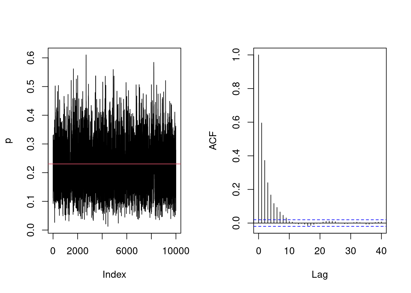
acceptance <- attempts <-0for(i inseq_len(B + burnin)){ ind <-pmax(1, i - burnin) # store values, then restard the counter# Run random walk par_cont[ind] <-univariate_rw_update(par_curr = par_cur, # current value of the parameterpar_name ="p", # name of the variable loglik = loglik, # log-likelihood functionlogprior = logprior, # log prior functionsd_prop = sd_prop, lb =0, # lower bound for the parameterub =1, # upper bound for the parametertransform =TRUE, # if lb/ub is provided, use transformationdata = data) # additional arguments passed to the functionif(par_cont[ind] != par_cur){ acceptance <- acceptance +1L #increment counter if move is accepted } attempts <- attempts +1L# Save current value par_cont[ind] -> par_curif(i %%100& i < burnin){# Adapt proposal every 100 iterations out <-adaptive(attempts = attempts, acceptance = acceptance, sd.p = sd_prop,target =0.44)# The function may return the values, or else change counters# We copy these sd_prop <- out$sd acceptance <- out$acc attempts <- out$att }}# Acceptance ratioprint(acceptance/attempts)
[1] 0.449
# Plot the Markov chain and the correlogrampar(mfrow =c(1,2))plot(par_cont, type ="l", ylab ="p")abline(h =mean(par_cont), col =2)acf(par_cont, main ="")
coda::effectiveSize(par_cont)/B
 var1
0.221
Compare now the results of using, instead of a logit transformation, a truncated normal kernel proposal.
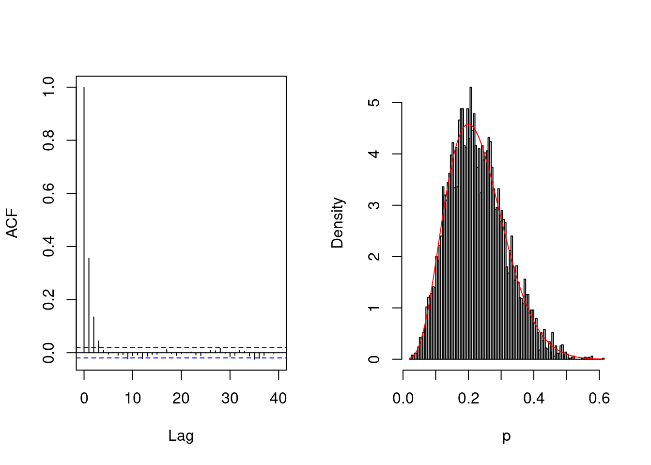
acceptance <-0# number of moves acceptedattempts <-0# number of proposalsfor(i inseq_len(B + burnin)){ ind <-pmax(1, i - burnin) # store values, then restard the counter# Run random walk par_cont[ind] <-univariate_rw_update(par_curr = par_cur, # current value of the parameterpar_name ="p", # name of the variable loglik = loglik, # log-likelihood functionlogprior = logprior, # log prior functionsd_prop = sd_prop, lb =0, # lower bound for the parameterub =1, # upper bound for the parametertransform =FALSE, # if lb/ub is provided, use transformationdata = data) # additional arguments passed to the functionif(par_cont[ind] != par_cur){ acceptance <- acceptance +1L #increment counter if move is accepted } attempts <- attempts +1L# Save current value par_cont[ind] -> par_curif(i %%100& i < burnin){# Adapt proposal every 100 iterations out <-adaptive(attempts = attempts, acceptance = acceptance, sd.p = sd_prop,target =0.44)# The function may return the values, or else change counters# We copy these sd_prop <- out$sd acceptance <- out$acc attempts <- out$att }}# Acceptance ratioprint(acceptance/attempts)
[1] 0.539
# Plot the Markov chain and the correlogrampar(mfrow =c(1,2))plot(par_cont, type ="l", ylab ="p")abline(h =mean(par_cont), col =2)acf(par_cont, main ="")
coda::effectiveSize(par_cont)/B
 var1
0.214
In this instance, the transformation leads to similar efficiency to using using truncated proposals. In both instances, we tuned the variance of the global proposal (Andrieu and Thoms 2008) to improve the mixing of the chains at approximate stationarity. This is done by increasing (decreasing) the variance if the historical acceptance rate is too high (respectively low) during burn-in period, and reinitializing after any change with an acceptance target of \(0.44\). We stop adapting to ensure convergence to the posterior after a suitable number of initial iterations.
Metropolis adjusted Langevin algorithm (MALA)
Since the posterior distribution is not available in closed-form, we resort to Markov chain Monte Carlo methods for sampling from it. Let \(p(\theta)\) denote the conditional (unnormalized) log posterior for a scalar parameter \(\theta \in (a, b)\). We considering a Taylor series expansion of \(p(\cdot)\) around the current parameter value at iteration \(t\), \(\theta^{(t)} \equiv\theta^{\text{curr}}\), \[\begin{align*}
p(\theta) = p(\theta^{\text{curr}}) + p'(\theta^{\text{curr}})(\theta - \theta^{\text{curr}}) + \frac{1}{2} p''(\theta^{\text{curr}})(\theta - \theta^{\text{curr}})^2 + \text{remainder}(\theta^{\text{curr}})
\end{align*}\] which suggests a Gaussian approximation with mean \(\mu^{\text{curr}} = \theta^{\text{curr}} - f'(\theta^{\text{curr}})/f''(\theta^{\text{curr}})\) and precision \(\tau^{-2} = -f''(\theta^{\text{curr}})\). We use truncated Gaussian distribution on \((a, b)\) with mean \(\mu\) and standard deviation \(\tau\), denoted \(\mathsf{TNo}(\mu, \tau, a, b)\) with corresponding density function \(q(\cdot; \mu, \tau, a, b)\). The Metropolis acceptance ratio for a proposal \(\theta^{\text{prop}} \sim \mathsf{TNo}(\mu^{\text{curr}}, \tau^{\text{curr}}, a, b)\) is \[\begin{align*}
\alpha = \frac{p(\theta^{\text{prop}})}{p(\theta^{\text{curr}})} \frac{ q(\theta^{\text{curr}} \mid \mu^{\text{prop}}, \tau^{\text{prop}}, a, b)}{q(\theta^{\text{prop}} \mid \mu^{\text{curr}}, \tau^{\text{curr}}, a, b)}
\end{align*}\] and we set \(\theta^{(t+1)} = \theta^{\text{prop}}\) with probability \(\min\{1, r\}\) and \(\theta^{(t+1)} = \theta^{\text{curr}}\) otherwise. To evaluate the ratio of truncated Gaussian densities \(q(\cdot; \mu, \tau, a, b)\), we need to compute the Taylor approximation from the current parameter value, but also the reverse move from the proposal \(\theta^{\text{prop}}\). Another option is to modify the move dictated by the rescaled gradient by taking instead \(\mu^{\text{curr}} = \theta^{\text{curr}} - \eta f'(\theta^{\text{curr}})/f''(\theta^{\text{curr}})\) proposal includes a tuning parameter, \(\eta \leq 1\), whose role is to prevent oscillations of the quadratic approximation, as in a Newton–Raphson algorithm. Relative to a random walk Metropolis–Hastings, the proposal automatically adjusts to the local geometry of the target, which guarantees a higher acceptance rate and lower autocorrelation for the Markov chain despite the higher evaluation costs. The proposal requires both \(f''(\theta^{\text{curr}})\) and \(f''(\theta^{\text{prop}})\) be positive, which shouldn’t be problematic in the vicinity of the mode.
We can use more efficient samplers by exploiting the geometry of the gradient and the hessian of the log posterior.
grad <-function(p, data, ...){ k <-sum(data) n <-length(data) k/p- (n-k)/(1-p)}hessian <-function(p, data, ...){ k <-sum(data) n <-length(data)-k/p^2- (n-k)/(1-p)^2}# Check gradient and Hessian matrix numericallynumDeriv::grad(func = loglik, data = data, x =0.1) -grad(data, p =0.1)
[1] -2.35e-10
max(abs(numDeriv::hessian(func = loglik, data = data, x =0.1) -hessian(data, p =0.1)))
[1] 8.08e-10
# Get derivative of beta prior using numerical differentiationgradprior <-function(p, data, ...){0}hessianprior <-function(p, data, ...){0}# Here, both functions are identically zero.
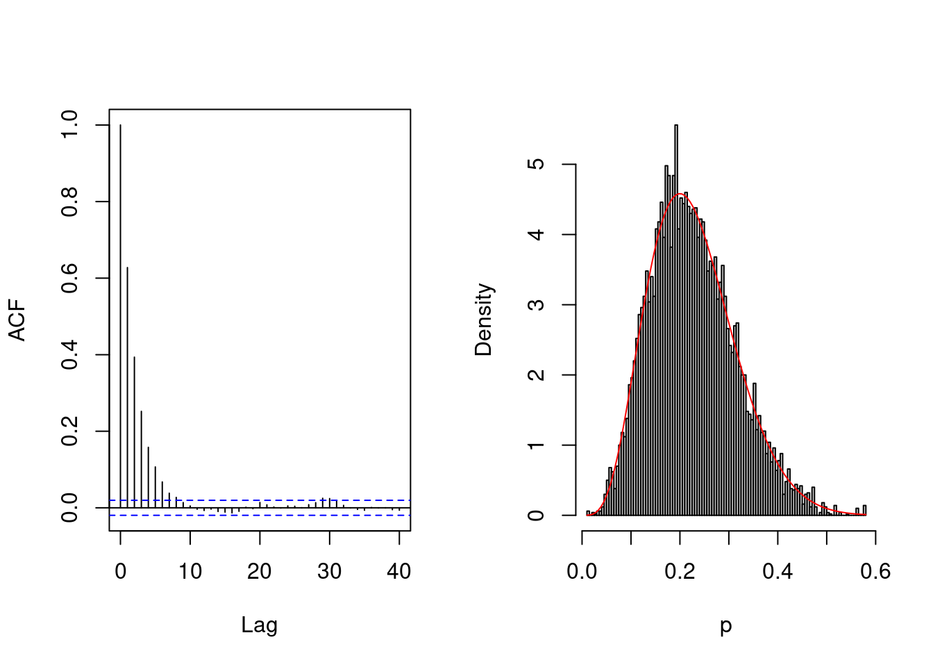
We begin with MALA, tuning the proposal variance to reach an acceptance rate of \(0.574\). This should reduce the autocorrelation by increasing the step size.
acceptance <- attempts <-0for(i inseq_len(B + burnin)){ ind <-pmax(1, i - burnin)# Run random walk par_cont[ind] <-univariate_mala_update(par_curr = par_cur, par_name ="p", # name of the variable loglik = loglik,logprior = logprior,loglik_grad = grad,logprior_grad =function(p, data, ...){0}, damping =0.5,sd_prop = sd_prop,transform =TRUE,lb =0,ub =1, # upper bounddata = data) # additional arguments passed to the functionif(par_cont[ind] != par_cur){ acceptance <- acceptance +1L } attempts <- attempts +1L# Save current value par_cont[ind] -> par_curif(i %%100& i < burnin){ out <-adaptive(attempts = attempts, acceptance = acceptance, sd.p = sd_prop,target =0.574) sd_prop <- out$sd acceptance <- out$acc attempts <- out$att }}
[1] 0.576
With a tuned-in variance to obtain an acceptance rate of 0.574, the effective sample size is 47% much higher than other proposals. The lag-one autocorrelation is 0.36.
for(i inseq_len(B)){# Run random walkpar_cont[i] <-univariate_laplace_update(par_curr = par_cur, par_name ="p", # name of the variable loglik = loglik, logprior = logprior,loglik_grad = grad,logprior_grad = gradprior, loglik_hessian = hessian,logprior_hessian = hessianprior,damping =1,lb =0,ub =1, # upper bounddata = data) # additional arguments passed to the function# Save current value par_cont[i] -> par_cur}
The acceptance rate is 76% with a lag-one autocorrelation of 0.63, but the effective sample size is 23%, much lower than for MALA. The advanced methods require additional calculations of the gradient and Hessian, the additional overhead of algorithms that exploit the geometry may or not be worth it.
Botev, Zdravko, and Pierre L’Écuyer. 2017. “Simulation from the Normal Distribution Truncated to an Interval in the Tail.”Proceedings of the 10th EAI International Conference on Performance Evaluation Methodologies and Tools on 10th EAI International Conference on Performance Evaluation Methodologies and Tools, 23–29. https://doi.org/10.4108/eai.25-10-2016.2266879.
Green, Peter J. 1995. “Reversible Jump Markov Chain Monte Carlo Computation and Bayesian Model Determination.”Biometrika 82 (4): 711–32. https://doi.org/10.1093/biomet/82.4.711.
Robert, Christian P., and George Casella. 2004. “The Metropolis—Hastings Algorithm.” In Monte Carlo Statistical Methods. Springer. https://doi.org/10.1007/978-1-4757-4145-2_7.
Roberts, Gareth O., and Jeffrey S. Rosenthal. 2001. “Optimal Scaling for Various Metropolis–Hastings Algorithms.”Statistical Science 16 (4): 351–67. https://doi.org/10.1214/ss/1015346320.
Sherlock, Chris. 2013. “Optimal Scaling of the Random Walk Metropolis: General Criteria for the 0.234 Acceptance Rule.”Journal of Applied Probability 50 (1): 1–15. https://doi.org/10.1239/jap/1363784420.
Stan Development Team. 2018. Stan Modeling Language Users Guide and Reference Manual. Version 2.9.0. http://mc-stan.org/.
Citation
BibTeX citation:
@online{belzile2023,
  author = {Belzile, Léo},
  title = {Strategies for {Markov} Chain {Monte} {Carlo} Algorithms},
  date = {2023-04-21},
  url = {https://lbelzile.bitbucket.io/posts/mcmc/},
  langid = {en}
}