Dong, Milholland, and Vijg (2016) claimed in a Nature paper that the maximum reported age at death has been decreasing, and that this result is significant. Their main finding is summarized in the following figure:

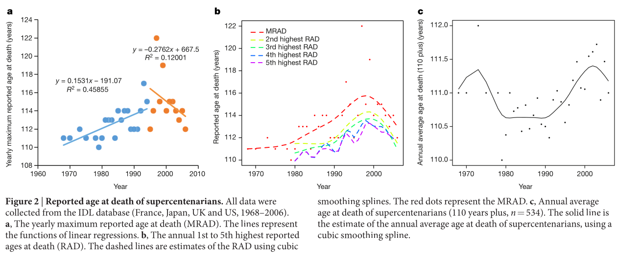
Figure 2 from Dong, Milholland, and Vijg (2016)

The latter shows (a) linear regressions of the maximum reported age at death over time, with a changepoint the year after Jeanne Calment died, (b) cubic smoothing splines fitted separately to the \(r=5\) largest order statistics in each year and (c) sample average of the age at death of supercentenarians, smoothing using a cubic smoothing spline.

While the problems with the statistical analyses have been reported elsewhere Rootzén and Zholud (2017), the purpose is this post to use recent International Database on Longevity (IDL) (French Institute for Demographic Studies 2023) to revisit some of the points of contention and highlight their impact on inference.

When it was added online in 2010, the IDL included records of supercentenarians (i.e., people who died above the age of 110 years) who died during a specified period of time, denoted \(c_1\) and \(c_2\). These calendar dates define the sampling frame, a form of interval truncation. Indeed, people who were born in year 1900, say, who survived beyond 2010 would not be included. Similarly, for earlier cohorts, only the oldest individuals born in year \(l\) would be alive if \(l-c_1 > 110\). If the rate at which people reach old age was the same, these two effects would counterbalance one another, but this is not the case here since mortality has decreased over the course of the century and the world population has increased, so many ghosts are found near \(c_2\).

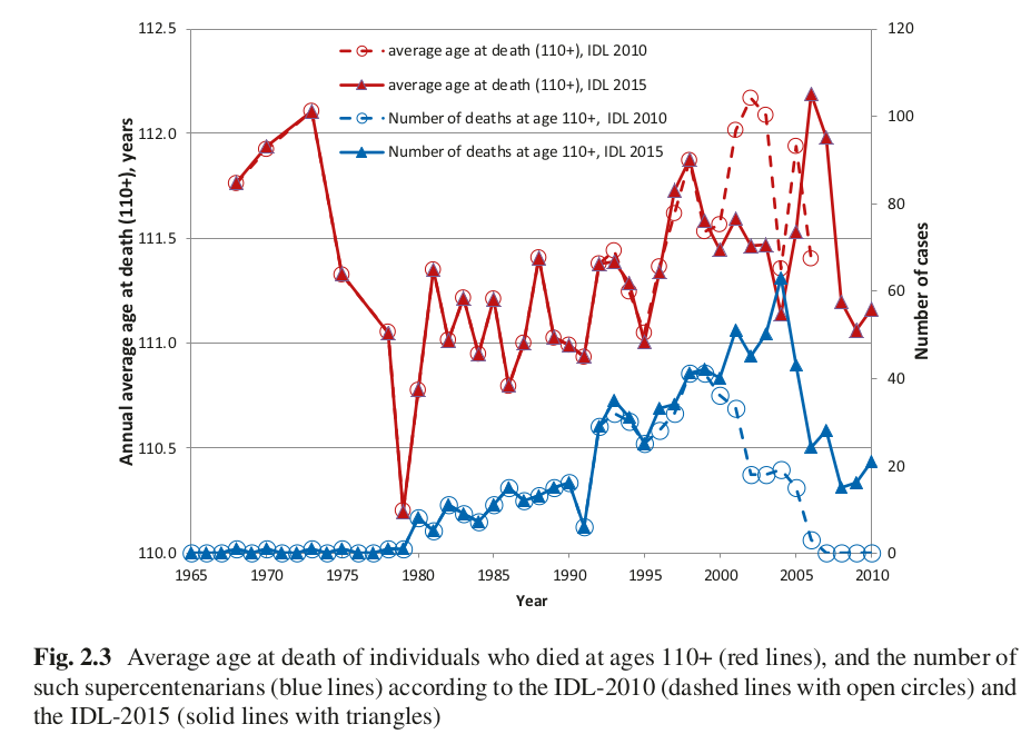
Dong, Milholland, and Vijg (2016) computed the sample age at death of people and the maximum reported age at death per birth year, sometimes referred to (incorrectly) as a birth cohort. As the IDL was augmented with more recent data, the pattern arising from the truncation disappears: this can be seen from Figure 2.3 from Jdanov, Shkolnikov, and Gellers-Barkmann (2021).

Changepoints

Dong, Milholland, and Vijg (2016) used two linear regression, splitting the data into two segments: before 1997 and after 1997. This year is notable because it is the age at which Jeanne Calment died. If data were independent and identically distributed (they aren’t), then we could indeed fit a linear regression and perform a Chow test (Chow 1960) to check. Choosing the maximum value is a form of selection mechanism, as it seems visually to be the point that maximizes the likelihood ratio statistic and the distribution is non-standard (Kim and Siegmund 1989). Brown, Albers, and Ritchie (2017) show that the downward trend would be removed altogether if we picked an earlier changepoint.

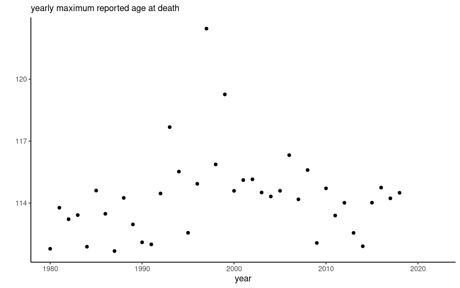
This approach is flawed from the start since the data are not identically distributed (due to truncation), the maximum of larger samples is stochastically larger than that of smaller samples (given the number of people over which we compute the maximum is different for each year) and the test procedure needs to account for the changepoint estimation. The truncation effects disappear if we consider longer collection period; for example, Figure 1 shows the data for France, England and Wales, USA and Japan from a more recent of the IDL (2023), showing indeed that much of the downward trend is gone.

Figure 1: Maximum reported age at death for France, England and Wales, USA and Japan based on IDL data from February 2023.

If we were to fit (incorrectly because it does not account for the truncation, nonstationarity of varying sample size for each year) a changepoint model with different intercept and slopes for year at death, we get:

changepoint <- chngpt::chngptm(
  formula.1 = MRAD ~ 1, 
  formula.2 = MRAD ~ DYEAR, 
  data = idl_sub |> mutate(DYEAR = DEATH_YEAR - 1980), 
  type = "stegmented", 
  family = "gaussian",
  var.type = "bootstrap",
  bootstrap.type = "wild",
  ci.bootstrap.size = 100L)
summary(changepoint)

Change point model threshold.type:  stegmented 

Coefficients:
                        est Std. Error*       (lower      upper)     p.value*
(Intercept)     111.0443293  0.23299674 110.68618013 111.5995274 0.0000000000
DYEAR             0.1323626  0.03895209   0.02327091   0.1759631 0.0006785841
DYEAR>chngpt      1.6593439  1.81340901  -3.84508591   3.2634774 0.3601700308
(DYEAR-chngpt)+  -0.2545795  0.12671462  -0.33566793   0.1610534 0.0445288691

Threshold:
       est Std. Error     (lower     upper) 
 15.000000   4.336735  11.000000  28.000000

While these results still fail to account for truncation and sample size, the ‘statistical significance’ is now gone.

Knots placement

The downward trend is mostly gone with the new data, but is less noticeable when we remove Jeanne Calment, would also be compensated if the data included Italy or more recent data from Japan (with reported people dying age 118 and 119). With limited data, the cubic smoothing splines shows noticeable artefacts of oversmoothing in Dong, Milholland, and Vijg (2016). The placement of the knots affects the conclusions drawn, as evidenced by automatic tuning in the right-hand panel of Figure 2, to be compared with equispaced knots in the left-hand panel.

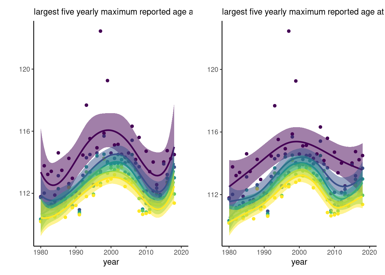
Figure 2: Largest 5 order statistics per year as a function of year of death, with cubic smoothing splines separately for each year based on a model with 5 knots (left) and with an automatic penalty based on the marginal likelihood (right).

We notice in Figure 2 that, after a dip early 2000s (attributable to the heatwave?), the trend is going back up. There are thus hardly evidence for the claimed decrease.

Further effects of truncation

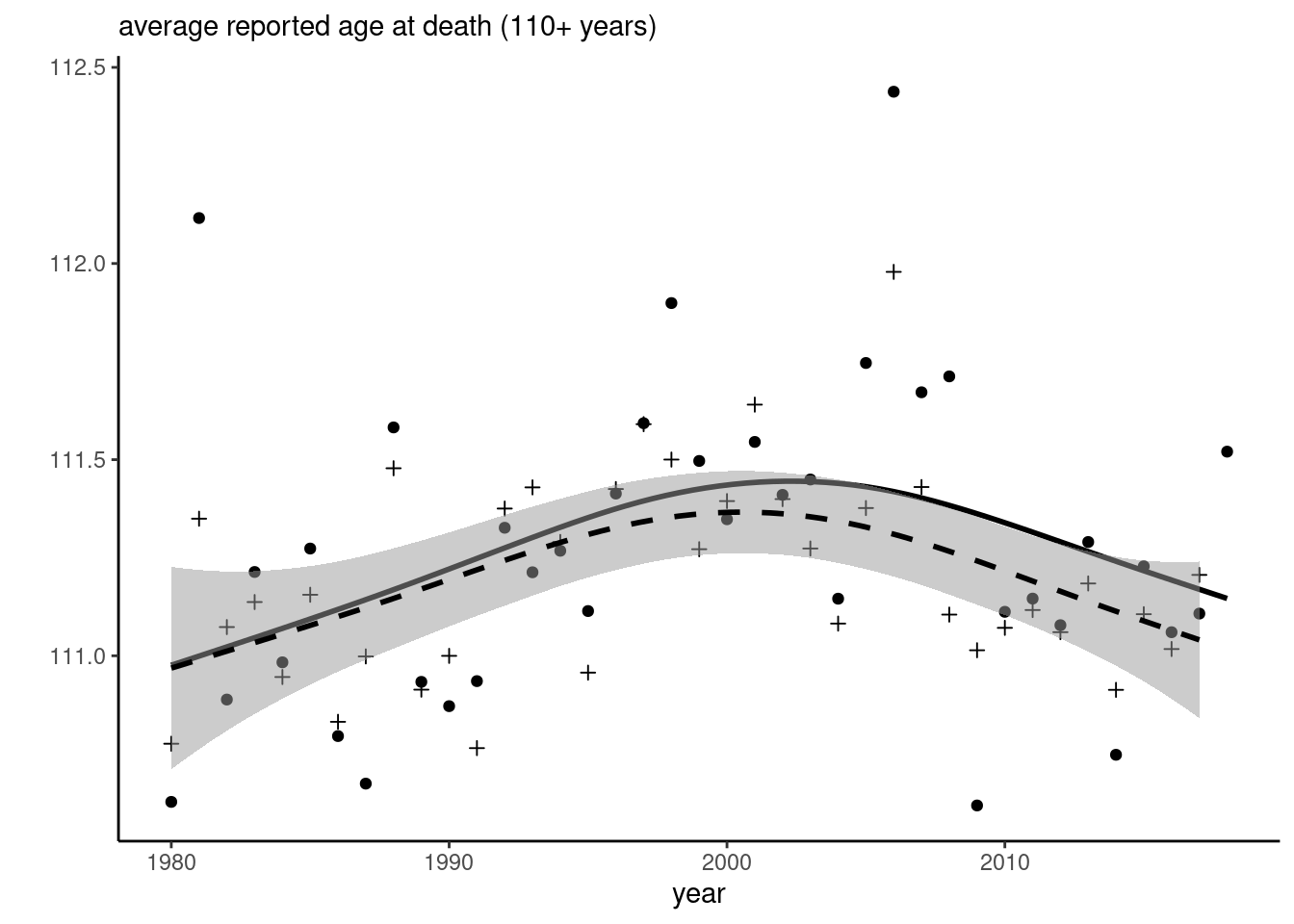
For positive random variables, we can estimate the expectation by computing the area under the survival curve. Since the sampling frame induces interval truncation and we seek to estimate the mean of the (untruncated) underlying distribution of excess lifetimes, we can instead use an EM algorithm to compute the nonparametric maximum likelihood estimator of the age at death and extract a mean estimator (Turnbull 1976). Figure 3 shows that the points are rather different from the sample mean and much less different, seeming to hover around a constant mean. We can also use the sample size as weighting in regression to draw a trend.

Figure 3: Average age at death of supercentenarians, with estimator based on empirical survival function integral (crosses) and the biased empirical averages (points). A cubic smoothing spline with automatic smoothing penalty for the former is overlaid with pointwise confidence intervals.

Conclusion

This post tried to demonstrate that much of the claim that there is a downward trend in the maximum age at death are based on flawed statistical analyses and that small tweaks and newer data can lead to much different conclusions, highlighting their lack of robustness. While there may have been a decrease and Jeanne Calment’s record is still very much an outlier today, the evidence does not hold to scrutinity.

References

Brown, Nicholas J. L., Casper J. Albers, and Stuart J. Ritchie. 2017. “Contesting the Evidence for Limited Human Lifespan.” Nature 546 (7660): E6–7. https://doi.org/10.1038/nature22784.

Chow, Gregory C. 1960. “Tests of Equality Between Sets of Coefficients in Two Linear Regressions.” Econometrica 28 (3): 591–605. http://www.jstor.org/stable/1910133.

Dong, Xiao, Brandon Milholland, and Jan Vijg. 2016. “Evidence for a Limit to Human Lifespan.” Nature 538 (7624): 257–59. https://doi.org/10.1038/nature19793.

French Institute for Demographic Studies, Ined (host). 2023. “International Database on Longevity.” https://www.supercentenarians.org/en/.

Jdanov, Dmitri A., Vladimir M. Shkolnikov, and Sigrid Gellers-Barkmann. 2021. “The International Database on Longevity: Data Resource Profile.” In Exceptional Lifespans, edited by Heiner Maier, Bernard Jeune, and James W. Vaupel, 22–24. Demographic Research Monographs. Cham, Switzerland: Springer.

Kim, Hyune-Ju, and David Siegmund. 1989. “The likelihood ratio test for a change-point in simple linear regression.” Biometrika 76 (3): 409–23. https://doi.org/10.1093/biomet/76.3.409.

Rootzén, H., and D. Zholud. 2017. “Human Life Is Unlimited — but Short (with Discussion).” Extremes 20 (4): 713–28.

Turnbull, Bruce W. 1976. “The Empirical Distribution Function with Arbitrarily Grouped, Censored and Truncated Data.” Journal of the Royal Statistical Society, Series B 38: 290–95.

Citation

BibTeX citation:

@online{belzile2023,
  author = {Belzile, Léo},
  title = {Trends in Longevity Records},
  date = {2023-02-28},
  url = {https://lbelzile.bitbucket.io/posts/trend-MRAD},
  langid = {en}
}

For attribution, please cite this work as:

Belzile, Léo. 2023. “Trends in Longevity Records.” February 28, 2023. https://lbelzile.bitbucket.io/posts/trend-MRAD.